Mapping Global Methane Emissions from Space with Deep Learning
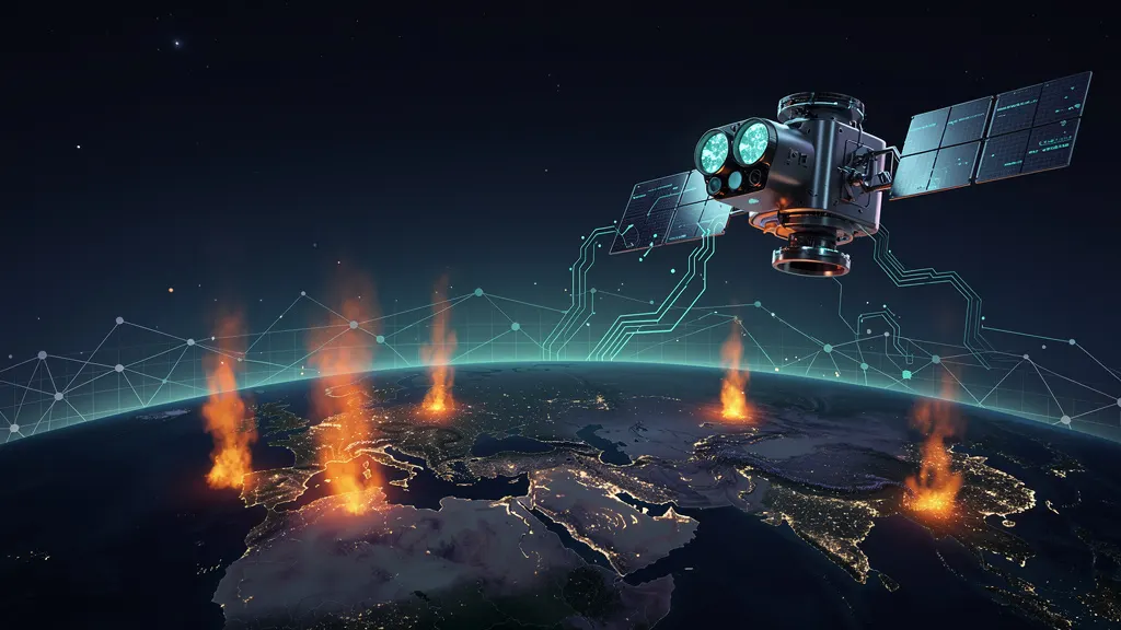
Google Research has published a detailed approach for mapping global methane emissions from space using deep learning. The method leverages satellite imagery to identify methane sources worldwide, providing a scalable tool for climate monitoring and emissions reduction efforts. By analyzing atmospheric data, the model detects plumes and enables more timely, transparent tracking of leaks across the planet.
Tags
Quick summary
Google Research has published a detailed approach for mapping global methane emissions from space using deep learning. The method leverages satellite imagery to identify methane sources worldwide, providing a scalable tool for climate monitoring and emissions reduction efforts. By analyzing atmospheric data, the model detects plumes and enables more timely, transparent tracking of leaks across the planet.
Mapping Global Methane Emissions from Space with Deep Learning
Methane is an invisible challenge. It escapes from wells, pipelines, landfills, and agricultural sites without a warning plume that our eyes can catch on conventional imagery. From orbit, however, the picture is different: satellites can register the spectral signatures of methane as it absorbs sunlight and re-emits infrared energy. The gap between the raw image and an accurate emission estimate is measurement science. The gap between millions of images and a global map is automation. Deep learning has become the key bridge across both.
This article walks through the technical ingredients of a methane-mapping system built on satellite data and neural networks. It mirrors the conceptual approach described by Google Research in its engineering post Mapping global methane emissions from space with deep learning, and then translates that concept into a practical, runnable workflow. We will look at why the problem is difficult, what deep learning contributes, and how you can set up your own inference pipeline with freely available tooling. All installation and usage examples are deliberately generic: they give you a functioning skeleton rather than pretending to reproduce any organization’s proprietary system.
The atmospheric problem
Carbon dioxide receives most of the attention in climate discussions, but methane is a harder short-term lever. It is a potent greenhouse gas with a comparatively short atmospheric lifetime, and its sources are scattered. Some emissions are large and continuous. Others are short-lived venting events that last only minutes. A monitoring system must therefore combine two attributes that rarely coexist in remote sensing: broad spatial coverage and high revisit frequency.
Satellites do not observe methane directly. They observe radiance in narrow spectral bands, and the presence of methane modifies that radiance in ways that can be converted into a concentration enhancement above the local background. The raw signal is small, and it can easily be corrupted by cloud edges, mineral surfaces, thermal noise, and the varying viewing geometry of individual overpasses. When the observations are averaged over a large region, a leak can become invisible. When they are examined at full resolution, the signal-to-noise ratio becomes a serious obstacle.
This is precisely the regime where a well-trained neural network outperforms classical thresholding. Instead of asking whether a single pixel exceeds a fixed value, the model can learn the spatial context of a plume: the bright core, the diffuse tail, the orientation downwind, and the surrounding terrain that should be treated as background. The output is no longer a binary flag but a structured map of likely plume locations.
Where deep learning changes the approach
The conventional satellite pipeline for trace-gas mapping runs through band ratios, absorption depth calculations, and expert-tuned thresholds. These methods are understandable and reproducible, but they struggle with the enormous diversity of scenes. A bare desert, a seasonally flooded rice paddy, a frozen lake, and a city rooftop all produce very different backgrounds. A fixed threshold calibrated on one scene type often fails on another.
Deep learning introduces several practical advantages:
- Contextual reasoning. A convolutional neural network sees a patch of pixels, not a single pixel. It can use the smooth gradient expected in a gas plume to reject speckle-like noise.
- Transferable representations. A model trained on one sensor can be fine-tuned on another with a fraction of the original dataset, which matters as new methane-observing missions come online.
- End-to-end calibration. Instead of separating the atmospheric correction from the detection step, the model can be trained to produce emission-related outputs directly from top-of-atmosphere reflectance, as long as the training labels are trustworthy.
- Uniform global analysis. A model applies the same decision boundary everywhere, which makes it feasible to scan terabytes of imagery and to surface only the most interesting events for human analysts.
None of these properties removes the need for careful preprocessing or independent validation. But they change the economics of analysis. A human analyst might inspect a few thousand scenes; an automated model can screen millions and route a few hundred ambiguous cases into a review queue.
None of these properties removes the need for careful preprocessing or independent validation. But they change the economics of analysis. A human analyst might inspect a few thousand scenes; an automated model can screen millions and route a few hundred ambiguous cases into a review queue.
Verified context for this article
The technical grounding for this discussion comes from a single accessible primary source: the Google Research blog post titled Mapping global methane emissions from space with deep learning (https://research.google/blog/mapping-global-methane-emissions-from-space-with-deep-learning), which was verified on 2026-09-01. The post is, as the title states, a research-blog narrative rather than a formal scientific paper. Where the present article moves beyond the blog’s general message, it does so in explicitly practical terms: the installation steps, data preparation routines, and code snippets below are educational examples that follow the same broad pattern, not representations of the original research implementation.
A practical mapping workflow
A complete methane-mapping system contains several distinct components that are useful to keep separate in your own project:
- Data acquisition. Satellite scenes arrive as multi-band GeoTIFFs or cloud-optimized archives, often with separate metadata files describing the atmospheric conditions and solar geometry.
- Preprocessing. Bands must be resampled to a common resolution, clouds must be masked, and radiance values should be converted into a comparable surface reflectance product.
- Detection. A segmentation model consumes image patches and produces a per-pixel probability that methane is present.
- Scene-level aggregation. Detections are clustered into plumes, and each plume is converted into a magnitude estimate and a location tag.
- Reporting and review. Results are written to GeoPackage, CSV, or an interactive map for analysts.
The remainder of this article focuses on components 1 through 4 with a lean, real setup.
Requirements
You will need the following:
- A Linux or macOS machine. Windows works with minor changes to the activation command.
- Python 3.10 or newer. We will create an isolated virtual environment.
- At least 12 GB of disk space for test scenes. Production-scale analysis needs far more.
- An NVIDIA GPU with at least 8 GB of VRAM is strongly recommended. The example inference script will run on CPU, but slowly.
The Python packages we will use are standard in the geospatial machine-learning ecosystem: rasterio for reading satellite images, numpy for array math, torch and torchvision for the model, and geopandas for writing vector outputs.
Step-by-step installation
First, create a virtual environment to keep dependencies isolated from the rest of your system.
python3 -m venv ~/.venvs/methane-mlActivate the environment. Every later command in this section assumes that you have run this activation line in the same shell.
source ~/.venvs/methane-ml/bin/activateUpgrade the basic packaging tools before installing anything else.
pip install --upgrade pip setuptools wheelInstall the core numerical and data-handling libraries.
pip install numpy pandas matplotlib requests pyyaml tqdmInstall PyTorch with CUDA support. If you do not have an NVIDIA GPU, replace the index URL with the CPU-only variant suggested on the official PyTorch site.
pip install torch torchvision --index-url https://download.pytorch.org/whl/cu121Install the geospatial readout and vector output libraries.
pip install rasterio shapely geopandasFinally, verify that the critical imports work. You should see no error messages after the imports, and the CUDA availability line will print False on a CPU-only machine.
python -c "import torch, rasterio; print(torch.__version__); print(torch.cuda.is_available())"Preparing a satellite scene
Satellite products arrive in many dialects, but the common denominator is a multi-band raster. The snippet below assumes you have already downloaded a region of interest and saved the relevant GeoTIFF files in a folder. It stacks the spectral bands that are sensitive to methane absorption, clips any invalid edge values, and resamples all bands to the coarsest resolution so that they lie on a common grid.
import rasterio
import numpy as np
from pathlib import Path

BANDS = ["B11", "B12", "B8A"]  # shortwave-infrared bands around methane absorption

def prepare_scene(scene_dir: Path):
    arrays, meta = [], None
    for name in BANDS:
        path = scene_dir / f"{name}.tif"
        with rasterio.open(path) as src:
            if meta is None:
                meta = src.meta.copy()
                meta.update(count=len(BANDS), dtype="float32")
            arrays.append(src.read(1).astype("float32"))

    stack = np.stack(arrays, axis=0)
    cloud_path = scene_dir / "cloud_mask.tif"
    if cloud_path.exists():
        with rasterio.open(cloud_path) as src:
            cloud = src.read(1).astype("bool")
        stack[:, cloud] = np.nan  # mask clouds before the model sees them

    with rasterio.open(scene_dir / "prepared.tif", "w", **meta) as dst:
        dst.write(stack)

    return scene_dir / "prepared.tif"
Note that the choice of B11, B12, and B8A matches Sentinel-2’s shortwave-infrared channels, which are commonly used for plume screening. If your source data uses a different spectral convention, you must update the list accordingly. The most reliable way to confirm usable bands is to inspect the scene metadata and compare the wavelength descriptions against methane absorption features.
A minimal segmentation model
Rather than writing a large U-Net from scratch, the example below uses a compact convolutional backbone that accepts a multi-band patch and returns a single-channel probability map. This is intentionally small enough to train or fine-tune on one GPU, but it is not the kind of production-grade architecture described in the research literature. Think of it as a baseline you can later replace.
import torch
import torch.nn as nn

class PlumeSegNet(nn.Module):
    def __init__(self, in_channels: int):
        super().__init__()
        self.encoder = nn.Sequential(
            nn.Conv2d(in_channels, 16, 3, padding=1), nn.ReLU(),
            nn.Conv2d(16, 32, 3, padding=1), nn.ReLU(),
            nn.MaxPool2d(2),
            nn.Conv2d(32, 64, 3, padding=1), nn.ReLU(),
            nn.Conv2d(64, 64, 3, padding=1), nn.ReLU(),
        )
        self.decoder = nn.Sequential(
            nn.Upsample(scale_factor=2, mode="bilinear", align_corners=False),
            nn.Conv2d(64, 32, 3, padding=1), nn.ReLU(),
            nn.Conv2d(32, 1, 1),
            nn.Sigmoid(),
        )

    def forward(self, x):
        return self.decoder(self.encoder(x))
This model outputs values between 0 and 1 for every pixel. During training, those values are compared against a binary mask prepared by an expert analyst or by an automatic labeling procedure. For the educational pipeline, you can store the checkpoint after training and reuse it for inference across new scenes.
Usage examples
Once the environment is ready, the model is defined, and a checkpoint exists, inference works in four steps. First, load the checkpoint and set the model to evaluation mode.
import torch

model = PlumeSegNet(in_channels=3)
checkpoint = torch.load("plume_checkpoint.pt", map_location="cpu")
model.load_state_dict(checkpoint["model_state_dict"])
model.eval()
Second, read the prepared scene in patches. Patch-based inference prevents out-of-memory failures on very large rasters.
import numpy as np
import rasterio
from rasterio.windows import Window

def predict_scene(prepared_path: str, patch_size: int = 256):
    with rasterio.open(prepared_path) as src:
        n_cols, n_rows = src.width, src.height
        result = np.zeros((n_rows, n_cols), dtype="float32")
        for row in range(0, n_rows, patch_size):
            for col in range(0, n_cols, patch_size):
                w = src.read(window=Window(col, row,
                                           min(patch_size, n_cols - col),
                                           min(patch_size, n_rows - row)))
                x = torch.from_numpy(w).unsqueeze(0)
                with torch.no_grad():
                    prob = model(x).squeeze(0).squeeze(0).numpy()
                h, ww = prob.shape
                result[row:row+h, col:col+ww] = prob
    return result
Third, extract plumes from the probability map as connected regions above a chosen threshold. The threshold should be tuned on validation data; 0.5 is only a starting point.
from scipy import ndimage

def extract_plumes(prob_map: np.ndarray, threshold: float = 0.5):
    binary = prob_map > threshold
    labeled, n_plumes = ndimage.label(binary)
    plumes = []
    for label_id in range(1, n_plumes + 1):
        ys, xs = np.where(labeled == label_id)
        plumes.append({
            "label": int(label_id),
            "pixels": int(len(xs)),
            "max_prob": float(prob_map[ys, xs].max()),
            "row_center": float(ys.mean()),
            "col_center": float(xs.mean()),
        })
    return plumes
Fourth, write the plumes and the probability map to disk so that a downstream analyst can review the detections in a GIS tool.
import json

with open("plumes.json", "w") as f:
    json.dump(plumes, f, indent=2)

with rasterio.open("prepared.tif") as src:
    profile = src.profile.copy()
    profile.update(dtype="float32", count=1, compress="deflate")
    with rasterio.open("probability.tif", "w", **profile) as dst:
        dst.write(prob_map, 1)
The full command line for a new scene would then look like this:
python prepare_scene.py data/scene_2025_08_14
python predict_scene.py data/scene_2025_08_14 --checkpoint plume_checkpoint.pt
python export_plumes.py data/scene_2025_08_14 --threshold 0.5
This three-step pattern has practical value beyond methane. By keeping the scene preparation independent from the model and exposing only a georeferenced input and output, you can later swap in a more powerful deep learning backbone or a completely different spectral band set without rewriting the entire system.
Limits and responsible interpretation
A model that detects patterns resembling plumes is not yet an emission inventory. Converting probability maps to tons per hour requires estimates of wind speed, wind direction, atmospheric transport, and the vertical distribution of the gas — information that a single satellite pass may not provide. Researchers frequently combine the plume detection step with a transport model or with simultaneous observations from a second instrument.
There are also sources of error that no amount of deep learning can eliminate. Clouds and sun glint remove data. Mountains cast shadows that mimic gradients. Urban infrastructure can produce spectral confusion. When a model is trained on one sensor, its performance on another must be reevaluated, especially if the spatial resolution differs by an order of magnitude.
The correct mindset for deployment is the human-in-the-loop model: machine learning finds candidate events, sorts them by confidence, and maintains a consistent global screening rule; analysts verify the shortlist, inspect the original imagery, and decide which events warrant ground-based follow-up. This arrangement uses the neural network where it is strongest — exhaustive and repeatable search — and keeps human judgment where it is required — final attribution and policy response.
For the practitioner, the open problems are therefore not only architectural. There is still no universal public benchmark that measures plume-detection performance across different sensors and terrain types. Creating such a benchmark, with carefully curated ground truth, would likely do more for the field than any single model improvement.
Conclusion
Mapping methane from space is a measurement problem wrapped in a scale problem. A satellite image contains enough evidence to localize a plume, but the amount of data exceeds the ability of manual analysis. Deep learning closes that gap by learning the spectral and spatial shape of plumes, then applying that knowledge consistently to every scene on the planet.
This article has walked through the logic behind that approach, grounded in the Google Research post on the subject, and provided a small but functional code path that you can run today: a Python environment with rasterio and torch, a multi-band scene preparation routine, a segmentation model, and a plume extraction script. The pieces are deliberately modular, because the real system that eventually produces a trusted global methane map will not be a single clever model. It will be a pipeline of careful data handling, honest validation, and machine learning used exactly where it adds value — at the frontier of scale.
Primary source: Mapping global methane emissions from space with deep learning, Google Research blog, https://research.google/blog/mapping-global-methane-emissions-from-space-with-deep-learning (verified 2026-09-01).